CONVOLUTIONAL NEURAL NETWORKS (CNN)

LIMITS OF FULLY CONNECTED LAYERS

Let’s assume that the feature detection layer need to compute some kind of local features (e.g. edges or keypoints) so the dimension of the $W$ array becomes:

$$size(W_l)=(3\times M\times N)\times (M\times N)$$

so the network’s layer dimensions increase exponentially with the image dimensions and becomes computationally impossible

CONVOLUTION TO THE RESCUE

Similarly to what is done in classical computer vision, where convolution is used to detect features in deep learning convolution can be used in layers to detect features with filters that are learned minimizing a loss function

CONVOLUTIONAL LAYERS

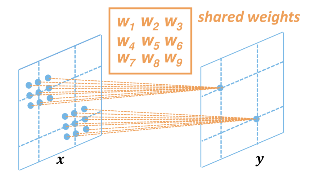
So to achieve this in a convolutional layer input and output are not flatten and each output is connected only to a local set of the input that shares the weights thus reducing the weights array dimension of the layer

$$y(i,j)=w_{1}x(i-1,j-1)+w_{2}x(i-1,j)+w_{3}x(i-1,j+1)+$$ $$w_{4}x(i,j-1)+w_{5}x(i,j)+w_{6}x(i,j+1)+$$ $$w_{7}x(i+1,j-1)+w_{8}x(i+1,j)+w_{9}x(i+1,j+1)\Rightarrow$$ $$y(i,j)=\sum _{m=-1}^{m=1}\sum _{l=-1}^{l=1}w(m,l)x(i+m,j+l)$$

COLOR IMAGE AS INPUTS

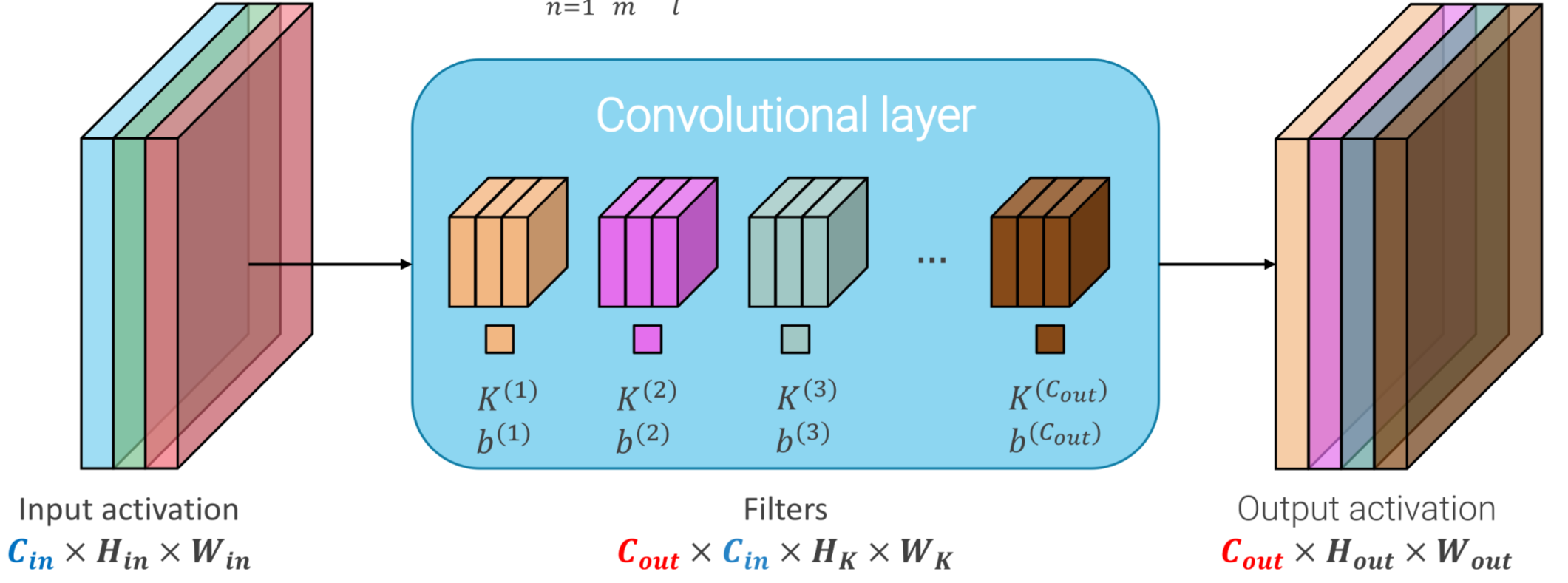
color images are represented as 3 channels input so convolution kernel must be 3-dimensional tensors

$$[K\times I](i,j)=\sum _{n=1}^3\sum _m\sum _l{K}_n(m,l)I_n(i+m,j+l)+b$$

OUTPUT ACTIVATION

By sliding the kernel over the image, input channel are translated in a single channel output i.e. the output activation of the convolutional layer, they are also called feature maps because layers tend to specialize in detecting specific features/patterns

MULTIPLE CHANNEL OUTPUT ACTIVATION

It can be useful to retrieve multiple channel output for detecting multiple features (e.g. horizontal and vertical edges)

$$[K^2\times I](i,j)=\sum _{n=1}^3\sum _m\sum _l{K}_n^2(m,l)I_n(i+m,j+l)+b^2$$

GENERAL STRUCTURE

This approach can be generalized, obtaining the general structure of a convolutional layer:

$$[K^k\times I](i,j)=\sum _{n=1}^{C_{in}}\sum _m\sum _l{K}_n^k(m,l)I_n(i+m,j+l)+b^{k}withk=\mathrm{1..}{C}_{out}$$

CHAINING CONVOLUTIONAL LAYERS

Convolutional layers are a form of linear transformation (they can be expressed by matrix) so in order to take advantage of network depth there is the need to chain them with some form of non-linearity (e.g. relu)

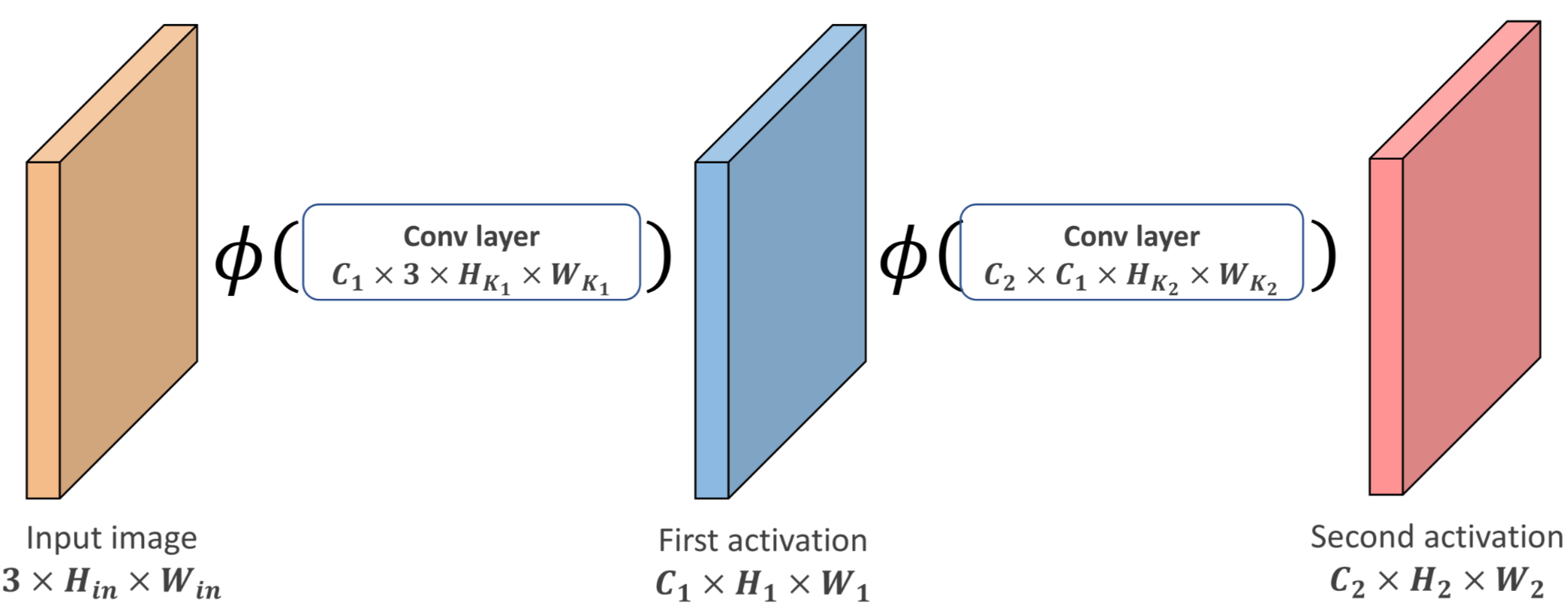
The main advantage of chaining is that with each level of depth the number of input pixels that the layer takes into account (e.g. the receptive field) gets larger and larger enabling the network to detect larger patterns

STRIDED CONVOLUTION

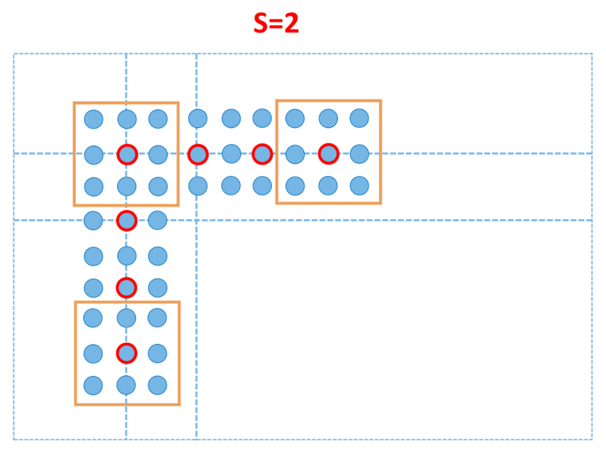
Convolution can be computed every $S$ (stride) positions in both directions

POOLING LAYERS

Pooling layers are layers with handcrafted functions that aggregates the input neighboring values in order to downsample the output

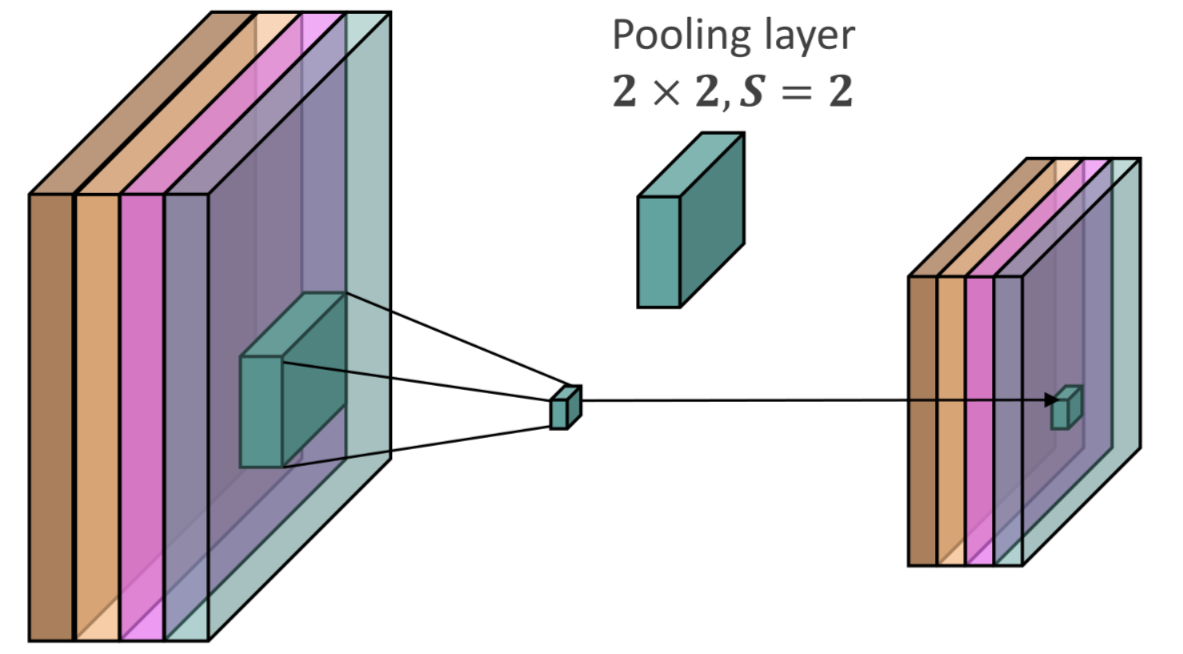
The pooling layer introduces some more hyperparameters such as dimensions of the kernel and stride

CNN FINAL STRUCTURE

Example of cnn’s can be LENET and ALEXNET

NUMBER OF LEARNABLE PARAMETERS

For a single convolutional layer the number of learnable parameter depends on kernel dimensions and input and output activation dimensions so the size of the $W$ array can be obtained as:

$$C_{out}\times (C_{in}\times H_k\times W_k+1)$$

THE PROBLEM WITH INCREASING DEPTH

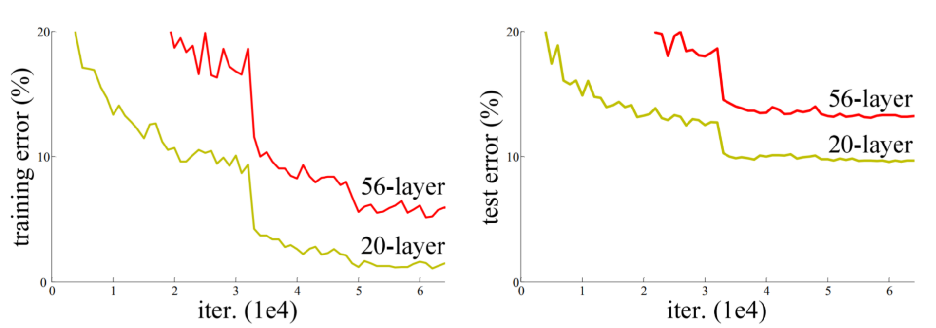
Intuitively increasing depth should take better results at the price of computation cost but as shown by VGG in real testing this is not the case

RESIDUAL LEARNING AS A SOLUTION

The idea is to add skip connection in order to fast forward the input to the deep nested layers

flowchart LR
A(input)
B[Conv]
C[BN]
D[ReLU]
E[Conv]
F[BN]
G((+))
H[ReLU]
A --> B --> C --> D --> E --> F --> G --> H
A --> G

So the output is given by:

$$H(x)=F(x)+x$$

An example of this can be found in RESNET

GLOBAL AVERAGE POOLING

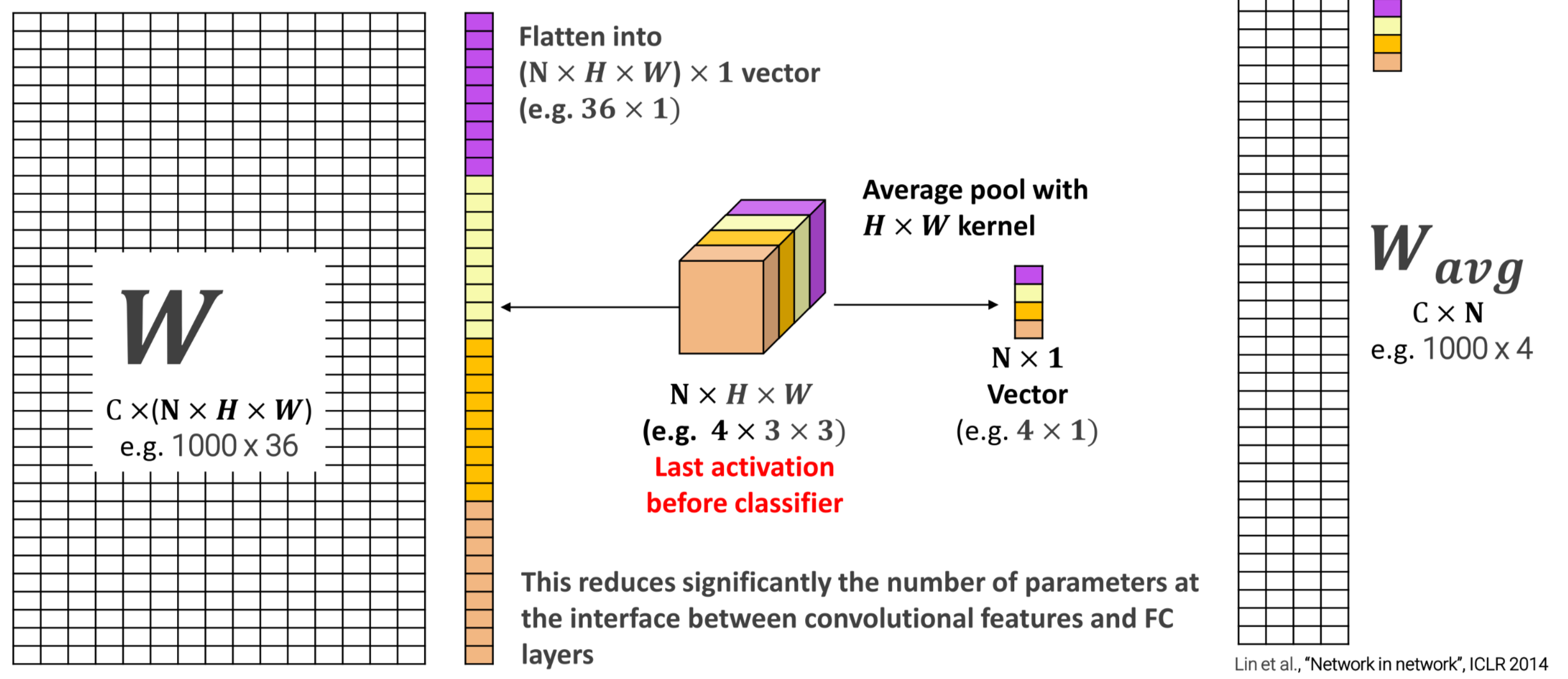
In order to reduce the number of parameter at the begin of the FC layers the output can be processed by average pooling

GROUPED CONVOLUTIONS

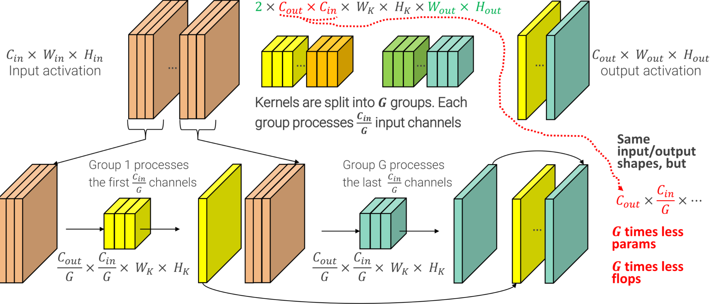
In order to improve the computational costs kernels are split into $G$ groups and each group process $\frac{C_{in}}{G}$ input channels, with this required flops and number of parameters are scaled by a $G$ factor

DEPTHWISE SEPARABLE CONVOLUTIONS

In order to improve the computational cost of convolution depthwise variant splits the spatial analysis and the feature combination and perform them sequentially.

flowchart TD
A[C X C X 3 X 3 Gconv + BN <br> G=C]
B[ReLU]
C[C X C X 1 X 1 + BN]
D[ReLU]
A --> B --> C --> D
START:::hidden --> A
D --> END:::hidden
classDef hidden display: none;

The first convolution step is realized as a GROUPED CONVOLUTIONS

TRANSFER LEARNING

To prevent overfitting, training of a deep neural network requires too big datasets that in a lot of deployment scenarios are expensive.

So in order to train big CNN a 2 steps approach is adopted:

• pre-train the deep network with a large, general purpose dataset
• fine-tune specific parts of the network with the smaller specific one dataset

PREVIOUS NEXT